[Part 2] Amplifying generalist research via forecasting – results from a preliminary exploration

This post covers the set-up and results from our exploration in amplifying generalist research using predictions, in detail. It is accompanied by a second post with a high-level description of the results, and more detailed models of impact and challenges. For an introduction to the project, see that post.

The rest of this post is structured as follows.

First, we cover the basic set-up of the exploration.

Second, we share some results, in particular focusing on the accuracy and cost-effectiveness of this method of doing research.

Third, we briefly go through some perspectives on what we were trying to accomplish and why that might be impactful, as well as challenges with this approach. These are covered more in-depth in a separate post.

Overall, we are very interested in feedback and comments on where to take this next.

Set-up of the experiment

A note on the experimental design

To begin with, we note that this was not an “experiment” in the sense of designing a rigorous methodology with explicit controls to test a particular, well-defined hypothesis.

Rather, this might be seen as an ”exploration” \[3\]. We tested several different ideas at once, instead of running a unique experiment for each separately. We also intended to uncover new ideas and inspiration as much as testing existing ones.

Moreover, we proceeded in a startup-like fashion where several decisions were made ad-hoc. For example, a comparison group was introduced after the first experiment had been completed; this was not originally planned, but later became evidently useful. This came at the cost of worsening the rigor of the experiment.

We think this trade-off was worth it for our situation. This kind of policy allows us to execute a large number of experiments in a shorter amount of time, quickly pivot away from bad ones, and notice low-hanging mistakes and learning points before scaling up good ones. This is especially helpful as we’re shooting for tail-end outcomes, and are looking for concrete mechanisms to implement in practice (rather than publishing particular results).

We do not see it as a substitute for more rigorous studies, but rather as a complement, which might serve as inspiration for such studies in the future.

To prevent this from biasing the data, all results from the experiment are public, and we try to note when decisions were made post-hoc.

Mechanism design

The basic set-up of the project is shown in the following diagram, and described below.

A two-sentence version would be:

Forecasters predicted the conclusions that would be reached by Elizabeth van Norstrand, a generalist researcher, before she conducted a study on the accuracy of various historical claims. We randomly sampled a subset of research claims for her to evaluate, and since we can set that probability arbitrarily low this method is not bottlenecked by her time.

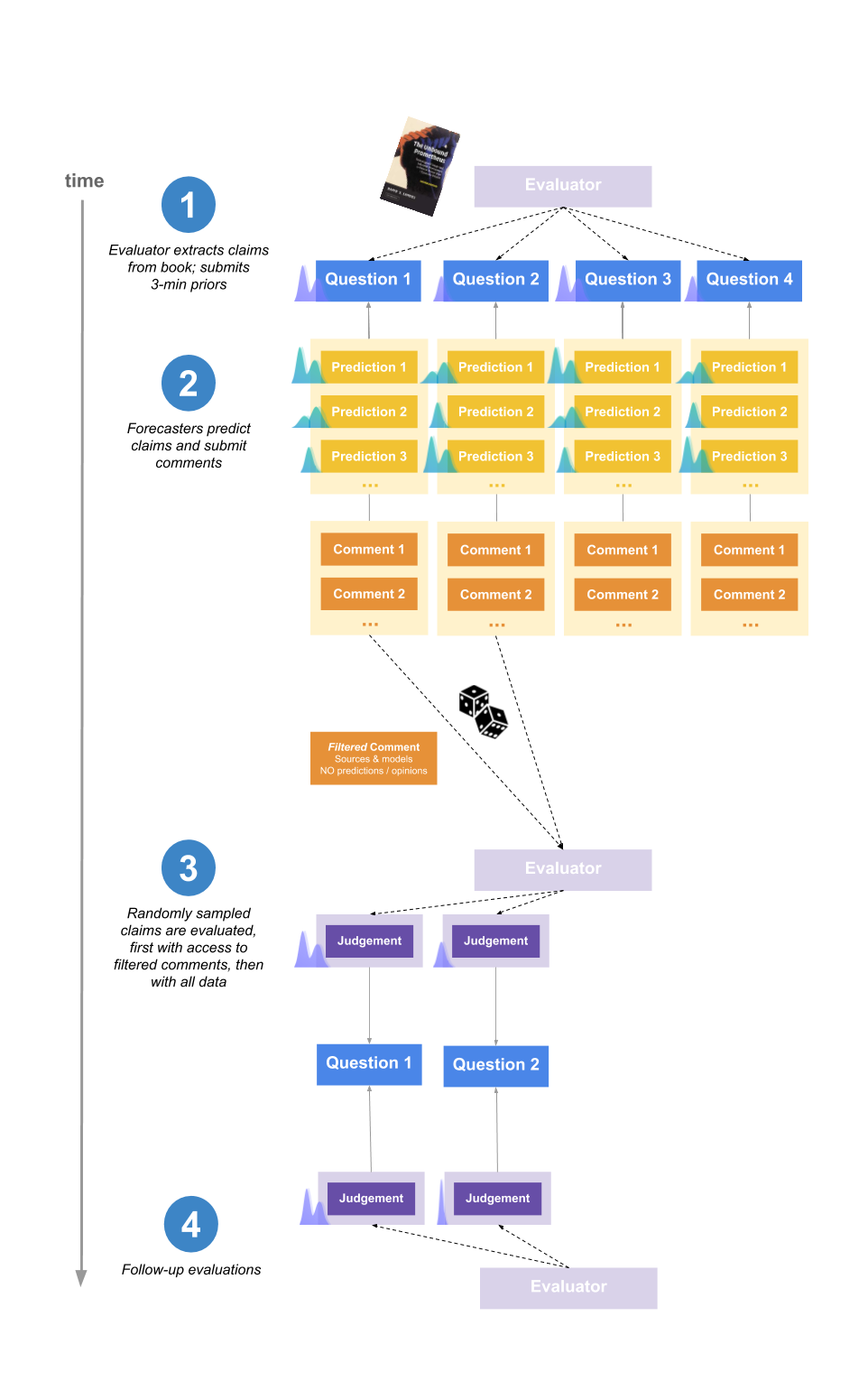
1. Evaluator extracts claims from the book and submits priors

The evaluator for the experiment was Elizabeth Van Norstrand, an independent generalist researcher known for her “Epistemic spot checks”. This is a series of posts assessing the trustworthiness of a book by evaluating some of it claims. We chose Elizabeth for the experiment as she has a reputation for reliable generalist research, and there was a significant amount of public data about her past evaluations of claims.

She picked 10 claims from the book The Unbound Prometheus: Technological Change and Industrial Development in Western Europe from 1750 to the Present, as well as a meta-claim about the reliability of the book as a whole.

All claims were assigned an importance rating from 1-10 based on their relevance to the thesis of the book as a whole. We were interested in finding if this would influence forecaster effort between questions.

Elizabeth also spent 3 minutes per claim submitting an initial estimate (referred to as a “prior”).

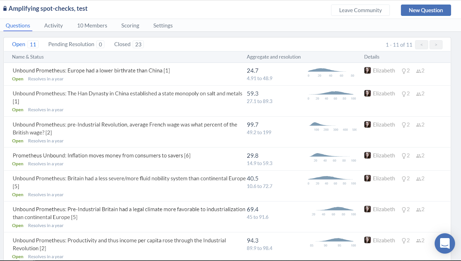
Beliefs were typically encoded as distributions over the range 0% to 100%, representing where Elizabeth expected the mean of her posterior credence in the claim to be after 10 more hours of research. For more explanation, see this footnote \[4\].

2. Forecasters make predictions

Forecasters predicted what they expected Elizabeth to say after ~45 minutes of research on the claim, and wrote comments explaining their reasoning.

Forecasters’ payments for the experiment were proportional to how much their forecasts outperformed the aggregate in estimating her 45-minute distributions. In addition, forecasters were paid a base sum just for participating. You can see all forecasts and comments here, and an interactive tool for visualising and understanding the scoring scheme here.

A key part of the design was that that forecasters did not know which question Elizabeth would randomly sample to evaluate. Hence they were incentivised to do their best on all questions (weighted by importance). This has the important implication that we could easily extend the amount of questions predicted by forecasters – even if Elizabeth can only judge 10 claims, we could have forecasting questions for 100 different claims \[5\].

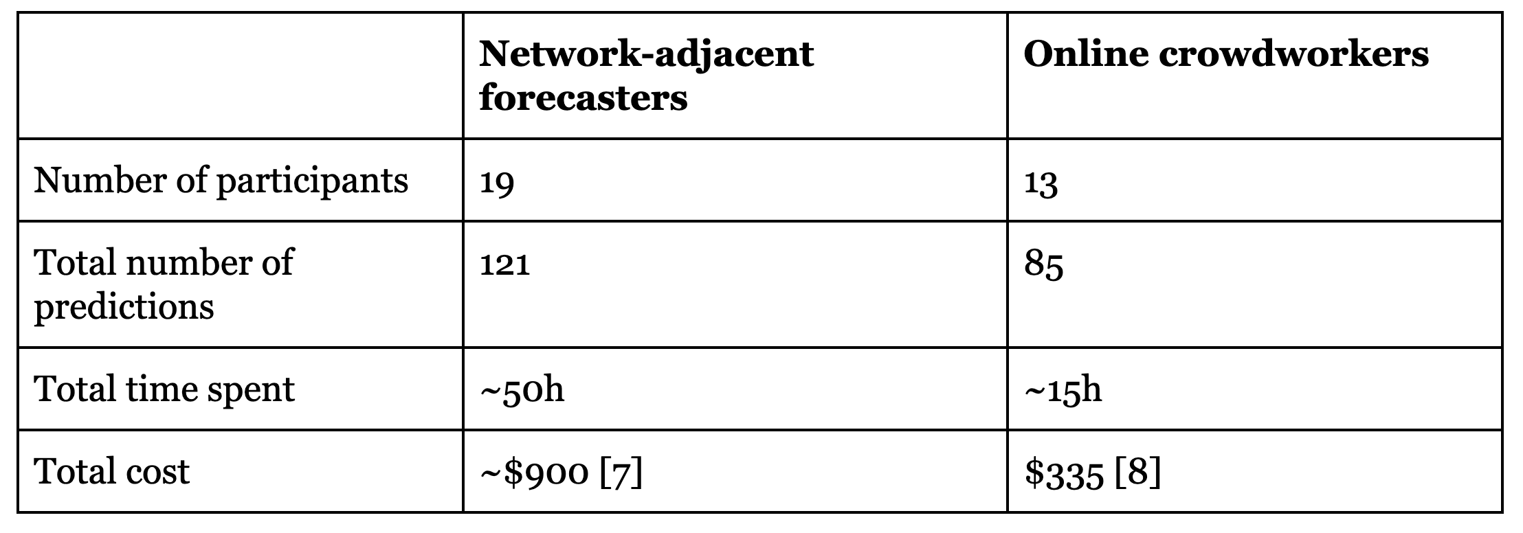
Two groups of forecasters participated in the experiment: one based on a mailing list with participants interested in participating in forecasting experiments (recruited from effective altruism-adjacent events and other forecasting platforms) \[6\], and one recruited from Positly, an online platform for crowdworkers. The former group is here called “Network-adjacent forecasters” and the latter “Online crowdworkers”.

3. The evaluator judges the claims

Elizabeth was given a time-budget of 6 hours, within which she randomly sampled claims to research and judge.

At this point, we wanted to use the work done by forecasters to help Elizabeth, while avoiding anchoring and biasing her with their estimates.

To solve this, Elizabeth was initially given a filtered version of the comments section for each claim, which contained all sources and models used, but which had been stripped of any explicit predictions or subjective opinion generalising from the data.

For example, for the question:

Pre-Industrial Britain had a legal climate more favorable to industrialization than continental Europe \[5\].

One commenter wrote:

Seems more likely to be true than not. The English Civil War and Glorious Revolution both significantly curtailed the arbitrary power of the monarch/gentry and raised the power of merchants in Britain, making likely that government was more favourable to mercantile interests. Hard to judge the claim about haggling.

And in Elizabeth’s initial briefing this was replaced by:

The English Civil War and Glorious Revolution both significantly curtailed the arbitrary power of the monarch/gentry and raised the power of merchants in Britain \[...\].

After arriving at a final estimate, Elizabeth was allowed to look at the full forecaster comments and predictions and optionally change her mind. In practice, she didn’t change her mind in any of these cases.

To summarise, the parts involved were:

• We summarised all of the relevant comments into a list and removed any descriptions that referred to people’s probabilities.
• We randomly chose 8 of the 10 claims for review by Elizabeth.
• Elizabeth saw this list, and spent 6 hours evaluating the 8 claims and resolving them with probability distributions of the values she expected to have for them in a future possible evaluation round. She divided this time in accordance to what seemed the most useful; for instance, questions with answers that became obvious quickly got a relatively small proportion of this time.
• Elizabeth got access to all predictions and all comments and was was allowed to change her resolutions. She decided not to in all of the cases.

4. The evaluator double-checks the evaluations

After having spent 6 hours researching 8 claims, Elizabeth randomly sampled two of those, each of which she spent an additional 3 hours researching. For the remaining claims, she waited until a week after the experiment, and then reread her notes and submitted new resolutions, to see if her way of converting beliefs into numbers was consistent over time. This part was intended to test the consistency and reliability of Elizabeth’s evaluations.

The outcome of this was that Elizabeth appeared highly consistent and reliable. You can see the data and graphs here. Elizabeth’s full notes explaining her reasoning in the evaluations can be found here.

Results and analysis

You can find all the data and interactive tools for exploring it yourself, here.

Online crowdworkers

We were interested in comparing the performance of our pool of forecasters to “generic” participants with no prior interest or experience forecasting.

Hence, after the conclusion of the original experiment, we reran a slightly modified form of the experiment with a group of forecasters recruited through an online platform that sources high quality crowdworkers (who perform microtasks like filling out surveys or labelinghttps://images.nunosempere.com/blog/2019/12/20/amplifying-general-research-via-forecasting-ii for machine learning models).

However, it should be mentioned that these forecasters were operating under a number of disadvantages relative to other participants, which means we should be careful when interpreting their performance. In particular:

• They did not know that Elizabeth was the researcher who created the claims and would resolve them, and so they had less information to model the person whose judgments would ultimately decide the questions.
• They did not use any multimodal or custom distributions, which is a way to increase tail-uncertainty and avoid large losses when forecasting with distributions. We expect this was because of the time-constraints set by their payment, as well as the general difficulty.

Overall the experiment with these online crowdworkers produced poor accuracy results at predicting Elizabeth’s resolutions (as is discussed further below).

Accuracy of predictions

This section analyses how well forecasters performed, collectively, in amplifying Elizabeth’s research.

The aggregate prediction was computed as the average of all forecasters' final predictions. Accuracy was measured using a version of the logarithmic scoring rule.

The following graph shows how the aggregate performed on each question:

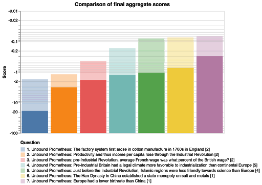
The opaque bars represent the scores from the crowdworkers, and the translucent bars, which have higher scores throughout, represent the scores from the network-adjacent forecasters. It’s interesting that the order is preserved, that is, that the question difficulty was the same for both groups. Finally we don’t see any correlation between question difficulty and the importance weights Elizabeth assigned to the questions.

However, the comparison is confounded by the fact that more effort was spent from the network-adjacent forecasters. The above graph also doesn’t compare performance to Elizabeth’s priors. Hence we also plot the evolution of the aggregate score over prediction number and time (the first data-point in the below graphs represent Elizabeth’s priors):

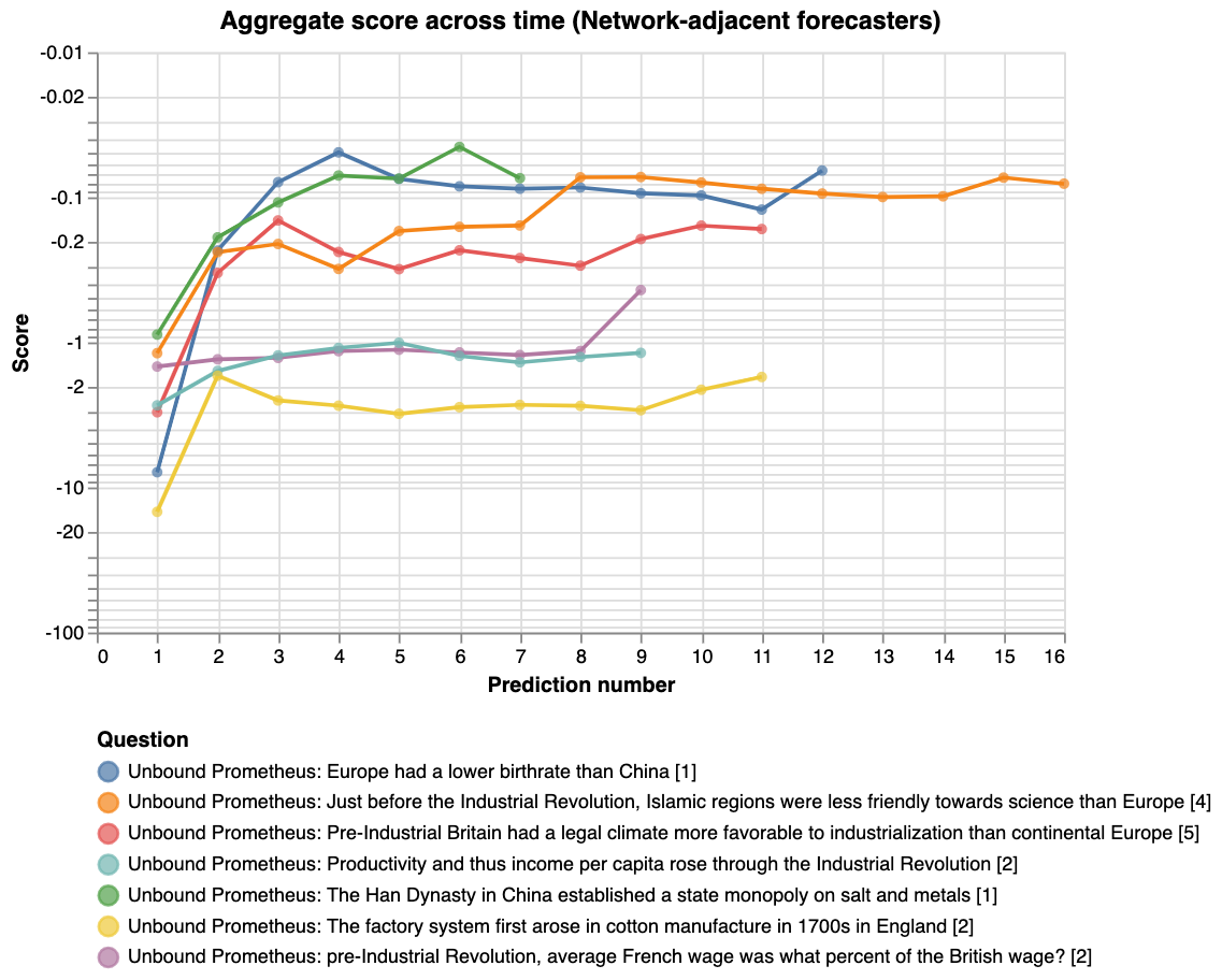
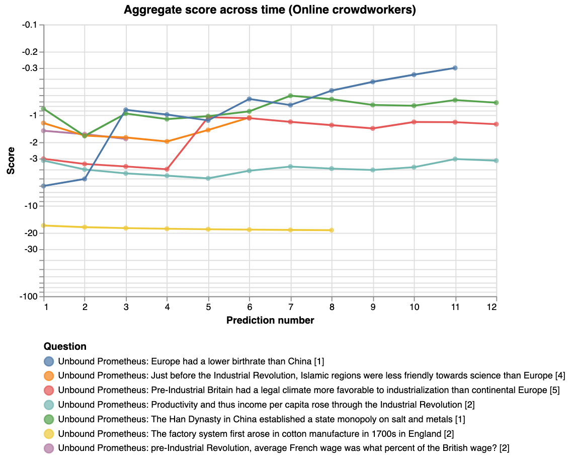
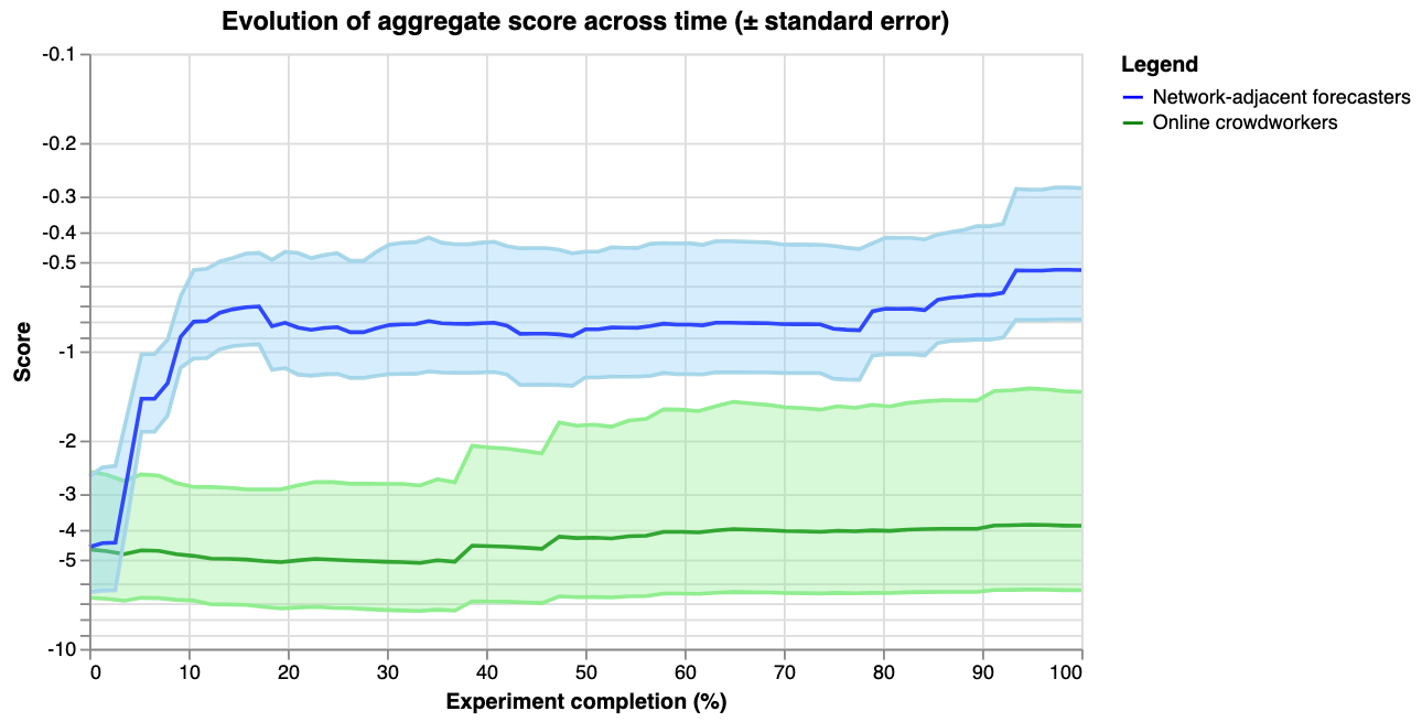
For the last graph, the y-axis shows the score on a logarithmic scale, and the x-axis shows how far along the experiment is. For example, 14 out of 28 days would correspond to 50%. The thick lines show the average score of the aggregate prediction, across all questions, at each time-point. The shaded areas show the standard error of the scores, so that the graph might be interpreted as a guess of how the two communities would predict a random new question \[10\].

One of our key takeaways from the experiment is that simple average aggregation algorithm performed surprisingly well, but only for the network-adjacent forecasters.

One way to see this qualitatively is by observing the graphs below, where we display Elizabeth’s priors, the final aggregate of the network-adjacent forecasters, and the final resolution, for a subset of questions \[11\].

Question examples

The x-axis \[12\] refers to the Elizabeth’s best estimate of the accuracy of a claim, from 0% to 100% (see section “Mechanism design, 1. Evaluator extracts claims” for more detail).

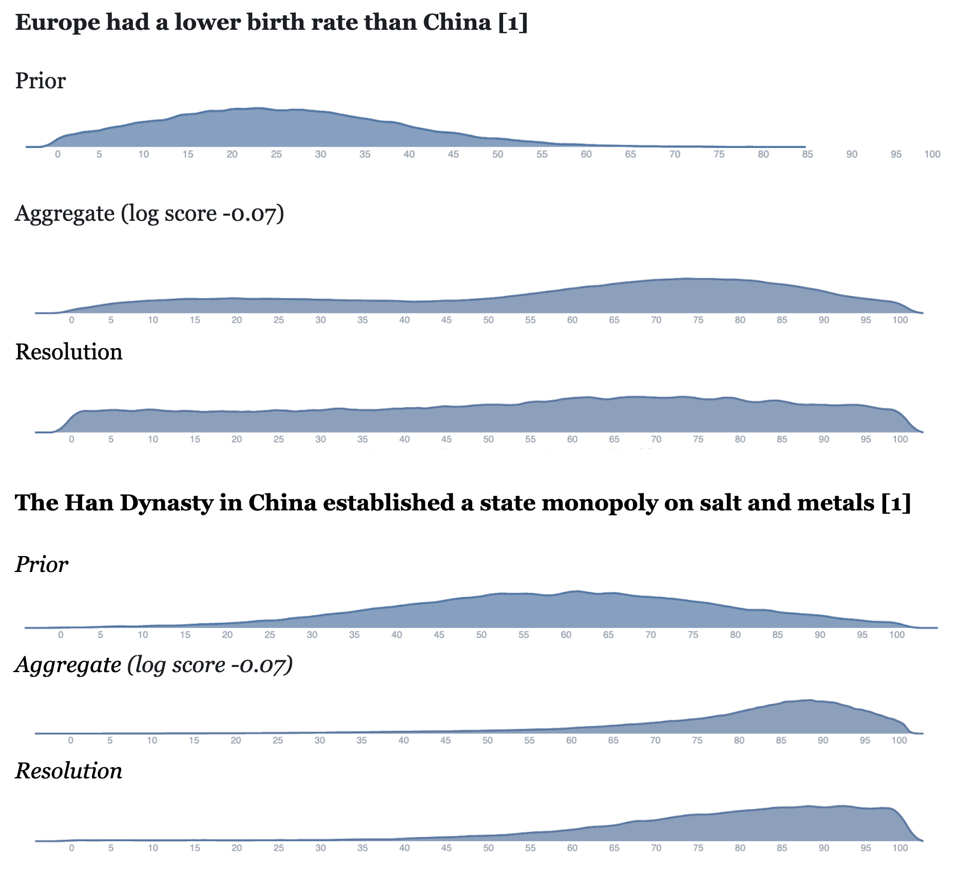
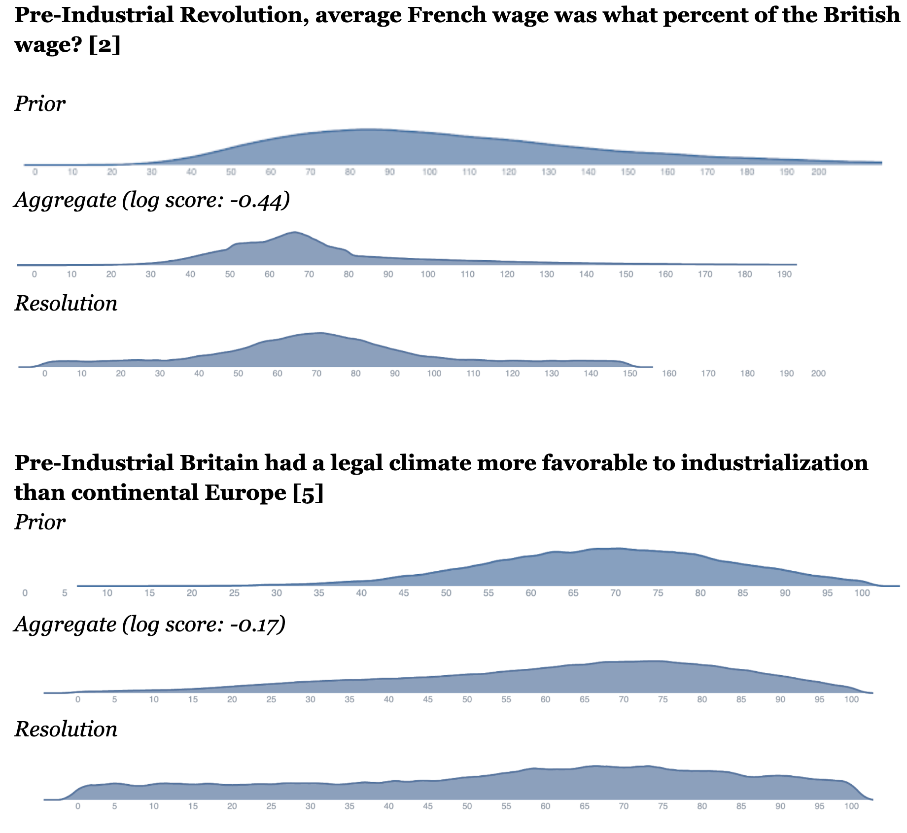
Another way to understand the performance of the aggregate is to note that the aggregate of network-adjacent forecasters had an average log score of -0.5. To get a rough sense of what that means, it’s the score you’d get by being 70% confident in a binary event, and being correct (though note that this binary comparison merely serves to provide intuition, there are technical details making the comparison to a distributional setting a bit tricky).

By comparison, the crowdworkers and Elizabeth’s priors had a very poor log score of around -4. This is roughly similar to the score you’d get if you predict an event to be ~5% likely, and it still happens.

Cost-effectiveness

High-level observations

This experiment was run to get a sense of whether forecasters could do a competent job forecasting the work of Elizabeth (i.e. as an “existence proof”). It was not meant to show cost-effectiveness, which could involve many efficiency optimizations not yet undertaken. However, we realized that the network-adjacent forecasting may have been reasonably cost-effective and think that a cost-effectiveness analysis of this work could provide a baseline for future investigations.

To compute the cost-effectiveness of doing research using amplification, we look at two measures: the information gain from predictors relative to the evaluator, and the cost of predictors relative to the evaluator.

Benefit/cost ratio = % information gain provided by forecasters relative to the evaluator / % cost of forecasters relative to the evaluator

If a benefit/cost ratio of significantly over 1 can be achieved, then this could mean that forecasting could be useful to partially augment or replace established evaluators.

Under these circumstances, each unit of resources invested in gaining information from forecasters has higher returns than just asking the evaluator directly.

Some observations about this.

First, note that this does not require forecasters to be as accurate as the evaluator. For example, if they only provide 10% as much value, but at 1% of the opportunity cost, this is still a good return on investment.

Second, amplification can still be worthwhile even if the benefit-cost ratio is < 1. In particular:

1. Forecasters can work in parallel and hence answer a much larger number of questions, within a set time-frame, than would be feasible for some evaluators.
2. Pre-work by forecasters might also improve the speed and quality of the evaluator’s work, if she has access to their research \[13\].
3. Having a low benefit-cost ratio can still serve as an existence proof that amplification of generalist research is possible, as long as the benefit is high. One might then run further optimised tests which try harder to reduce cost.

Results

The opportunity cost is computed using Guesstimate models linked below, based on survey data from participants collected after the experiment. We are attempting to include both hourly value of time and value of altruistic externalities. We did not include the time that our own team spent figuring out and organising this work.

For example, the estimated cost ratio for the network-adjacent forecasters in this experiment was 120%, meaning that the cost of obtaining a final aggregate prediction for a question was 20% higher when asking this group of 19 forecasters than when asking Elizabeth directly, all things considered.

The value is computed using the following model (interactive calculation linked below). We assume Elizabeth is an unbiased evaluator, and so the true value of a question is the mean of her resolution distribution. We then treat this point estimate as the _true_resolution, and compare to it the scores of Elizabeth’s resolution, had it been a prediction, vs. her initial prior; and the final aggregate vs. her initial prior. All scores are weighed by the importance of the question, as assigned by Elizabeth on a 1-10 scale \[14\].

Results were as follows.

(Links to models: network-adjacent cost ratio and value ratio, online crowdworker cost ratio and value ratio.)

The negative value ratio for the control group indicates that they assigned a lower probability to the mean of Elizabeth’s resolution than she her herself did when submitting her prior. Hence just accepting the means from those forecasts would have made us worse off, epistemically, than trusting the priors.

This observation is in tension with the some of the above graphs, which show a tiny increase in average log score between crowdworkers and Elizabeth’s priors. We are somewhat uncertain about the reason for this, though we think it is as follows: they were worse at capturing the resolution means than the prior, but they were sometimes better at capturing the resolution distribution (likely by the average of them adding on more uncertainty). And the value ratio only measures the former of those improvements.

Another question to consider when thinking about cost-effectiveness is diminishing returns. The following graph shows how the information gain from additional predictions diminished over time.

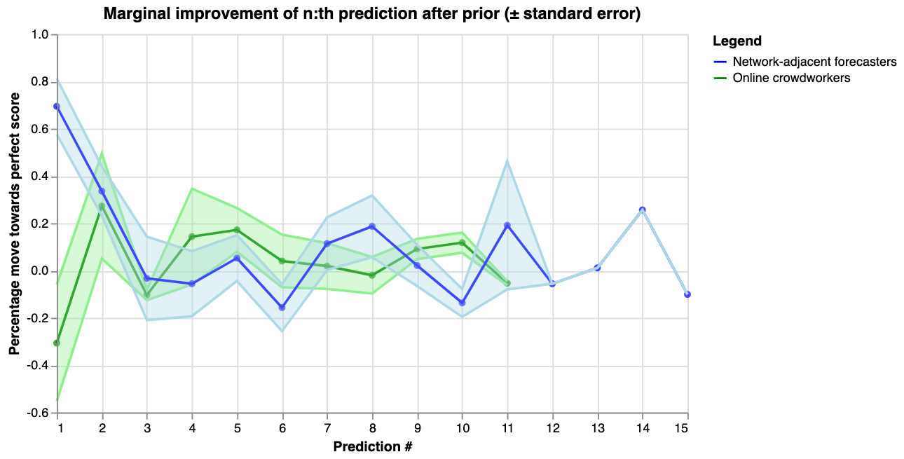
The x-axis shows the number of predictions after Elizabeth’s prior (which would be prediction number 0). The y-axis shows how much closer to a perfect score each prediction moved the aggregate, as a percentage of the distance between the previous aggregate and the perfect log score of 0 \[15\].

We observe that for the network-adjacent forecasters, the majority of value came from the first two predictions, while the online crowdworkers never reliably reduced uncertainty. Several hypotheses might explain this, including that:

• The first predictor on most questions was also one of the best participants in the experiment
• Most of the value of the predictors came from increasing uncertainty, and already after averaging 2-3 distributions we had gotten most of the effect there
• Later participants were anchored by the clearly visible current aggregate and prior predictions

Future experiments might attempt to test these hypotheses.

Perspectives on impact and challenges

This section summarises some different perspectives on what the current experiment is trying to accomplish and why that might be exciting, as well as some of the challenges it faces. To keep things manageable, we simply give a high-level overview here and discuss each point in more detail in a separate post.

There are several perspectives here given that the experiment was designed to explore multiple relevant ideas, rather than testing a particular, narrow hypothesis.

As a result, the current design is not optimising very strongly for any of these possible uses, and it is also plausible that its impact and effectiveness will vary widely between uses.

Perspectives on impact

• Mitigating capacity bottlenecks. The effective altruism and rationality communities face rather large bottlenecks in many areas, such as allocating funding, delegating research, vetting talent and reviewing content. The current setup might provide a means of mitigating some of those – a scalable mechanism of outsourcing intellectual labor.
• A way for intellectual talent to build and demonstrate their skills. Even if this set-up can’t make new intellectual progress, it might be useful to have a venue where junior researchers can demonstrate their ability to predict the conclusions of senior researchers. This might provide an objective signal of epistemic abilities not dependent on detailed social knowledge.
• Exploring new institutions for collaborative intellectual progress. Academia has a vast backlog of promising ideas for institutions to help us think better in groups. Currently we seem bottlenecked by practical implementation and product development.
• Getting more data on empirical claims made by the Iterated Amplification AI alignment agenda. These ideas inspired the experiment. (However, our aim was more practical and short-term, rather than looking for theoretical insights useful in the long-term.)
• Exploring forecasting with distributions. Little is known about humans doing forecasting with full distributions rather than point estimates (e.g. “79%”), partly because there hasn’t been easy tooling for such experiments. This experiment gave us some cheap data on this question.
• Forecasting fuzzy things. A major challenge with forecasting tournaments is the need to concretely specify questions; in order to clearly determine who was right and allocate payouts. The current experiments tries to get the best of both worlds – the incentive properties of forecasting tournaments and the flexibility of generalist research in tackling more nebulous questions.
• Shooting for unknown unknowns. In addition to being an “experiment”, this project is also an “exploration”. We have an intuition that there are interesting things to be discovered at the intersection of forecasting, mechanism design, and generalist research. But we don’t yet know what they are.

Challenges and future experiments

• Complexity and unfamiliarity of experiment. The current experiment had many technical moving parts. This makes it challenging to understand for both participants and potential clients who want to use it in their own organisations.
• Trust in evaluations. The extent to which these results are meaningful depends on your trust in Elizabeth Van Nostrand’s ability to evaluate questions. We think is partly an inescapable problem, but also expect clever mechanisms and more transparency to be able to make large improvements.
• Correlations between predictions and evaluations. Elizabeth had access to a filtered version of forecaster comments when she made her evaluations. This introduces a potential source of bias and a “self-fulfilling prophecy” dynamic in the experiments.
• Difficulty of converting mental models into quantitative distributions. It’s hard to turn nuanced mental models into numbers. We think a solution is to have a “division of labor”, where some people just build models/write comments and others focus on quantifying them. We’re working on incentive schemes that work in this context.
• Anti-correlation between importance and “outsourceability”. The intellectual questions which are most important to answer might be different from the ones that are easiest to outsource, in a way which leaves very little value on the table in outsourcing.
• Overhead of question generation. Creating good forecasting questions is hard and time-consuming, and better tooling is needed to support this.
• Overly competitive scoring rules. Prediction markets and tournaments tend to be zero-sum games, with negative incentives for helping other participants or sharing best practices. To solve this we’re designing and testing improved scoring rules which directly incentivise collaboration.

Footnotes

\[1\] Examples include: AI alignment, global coordination, macrostrategy and cause prioritisation.

\[2\] We chose the industrial revolution as a theme since it seems like a historical period with many lessons for improving the world. It was a time of radical change in productivity along with many societal transformations, and might hold lessons for future transformations and our ability to influence those.

\[3\] Some readers might also prefer the terms “integration experiment” and “sandbox experiment”.

\[4\] In traditional forecasting tournaments, participants state their beliefs in a binary event (e.g. “Will team X win this basketball tournament?”) using a number between 0% and 100%. This is referred to as a credence, and it captures their uncertainty in a quantitative way. The terminology comes from Bayesian probability theory, where rational agents are modelled as assigning credences to claims and then updating those credences on new information, in a way uniquely determined by Bayes’ rule. However, as a human, we might not always be sure what the right credence for a claim is. If I had an unlimited time to think, I might arrive at the right number. (This is captured by the “after 10 more hours of research” claim.) But if I don’t have a lot of time, I have some uncertainty about exactly how uncertain I should be. This is reflected in our use of distributions.

\[5\] In scaling the number of claims beyond what Elizabeth can evaluate, we would also have to proportionally increase the rewards.

\[6\] Many of these participants had previous experience with forecasting, and some were “superforecaster-equivalents” in terms of their skill. Others had less experience with forecasting but were competent in quantitative reasoning. For future experiments, we ought to survey participants about their previous experience.

\[7\] The payments were doubled after we had seen the results, as the initial scoring scheme proved too harsh on forecasters.

\[8\] The incentive schemes looked somewhat different between groups, mostly owing to the fact that we tried to reduce the complexity necessary to understand the experiment for the online crowdworkers, who to our knowledge had no prior experience with forecasting. They were each paid at a rate of ~$15 an hour, with the opportunity for the top three forecasters to receive a bonus of $35.

\[9\] Elizabeth did this by copying the claims into a google doc, numbering them, and then using Google random number generator to pick claims. For a future scaled up version of the experiment, one could use the public randomness beacon as a transparent and reproducible way to sample claims.

\[10\] In analysing the data we also plotted 95% confidence intervals by multiplying the standard error by 1.96. In that graph the two lines intersect for something like 80%-90% of the x-axis. You can plot and analyse them yourself here.

\[11\] We only display the first four resolutions to not too make up too much space (which were randomly chosen in the course of the experiment). All resolution graphs can be found here.

\[12\] The distributions are calculated using Monte Carlo sampling and Kernel smoothing, so are not perfectly smooth. This also led to errors around bounds being outside of the 0 to 100 range.

\[13\] For this experiment, Elizabeth informally reports that the time saved ranged from 0-60 minutes per question, but she did not keep the kind of notes required to estimate an average.

\[14\] This is a rough model of calculating this and we can imagine there being better ways of doing it. Suggestions are welcome.

\[15\] Using this transformation allows us to visualise the fact smaller scores obtained later in the contest can still be as impressive as earlier scores. For example, moving from 90% confidence to 99% confidence takes roughly as much evidence as moving from 50% to 90% confidence. Phrased in terms of odds ratios, both updates involve evidence of strength roughly 10:1.

Participate in future experiments or run your own

Foretold.io was built as an open platform to enable more experimentation with prediction-related ideas. We have also made data and analysis calculations from this experiment publicly available.

If you’d like to:

• Run your own experiments on other questions
• Do additional analysis on this experimental data
• Use an amplification set-up within your organisation

We’d be happy to consider providing advice, operational support, and funding for forecasters. Just comment here or reach out to this email.

If you’d like to participate as a forecaster in future prediction experiments, you can sign-up here.

Acknowledgements

Funding for this project was provided by the Berkeley Existential Risk Initiative and the EA Long-term Future Fund.

We thank Beth Barnes and Owain Evans for helpful discussion.

We are also very thankful to all the participants.